Jupyter Notebook is a web-based application for interactive work on Jupyter Notebook documents. These documents can combine source code, the source code’s output, and further text and images.

The system is accessible via a web browser. The Jupyter Notebook software connects a notebook document with an R or Python interpreter to allow interactive execution of the source code.

The software comes with preinstalled interpreters and a set of basic libraries for Python 2.7, Python 3.6, and R 3.6 in a multiuser configuration called Jupyterhub. These environments are named “Anaconda-Python2.7”, “Anaconda-Python3.6”, and “R”.

Users cannot modify this basic set of libraries. Instead, users can create own environments for Python 2.7 or Python 3.6, which are stored in the user’s home folder, and add additional libraries therein. For R, users can extend the basic library set, by installing additional libraries in a local package repository, which also stored in the user’s home folder.

A central instance of the Jupyter Notebook Server is available under https://jupyterhub.awi.de for all users with a valid AWI account. Personal instances of Jupyterhub are available for users or workgroups on request. They have a limited life span, after which they are deleted automatically. Own environments, as described before, remain, as they are stored in the user’s home folder, and will be available in all instances of Jupyterhub at AWI.

Working with the Jupyterhub System

The system is used by a web interface in the browser. After login, the interface offers four tabs, described below: “Files”, “Running”, “Clusters”, and “Conda”.

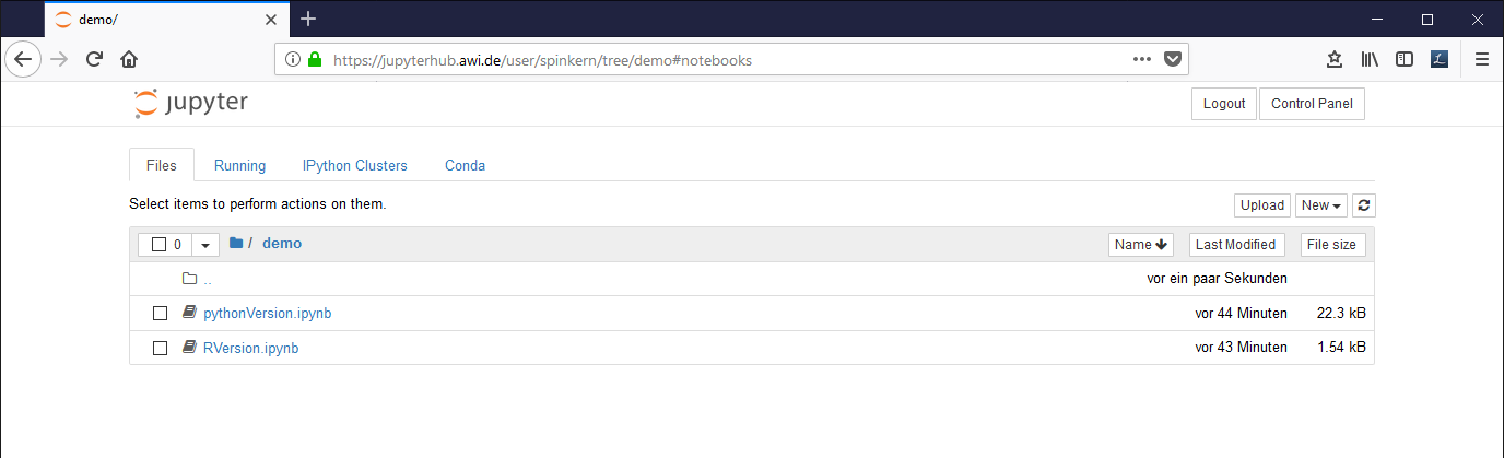
The “Files” tab

This tab shows a folder listing of the user’s home folder and offers a simple file browser including up- and download functionality.

It is not possible to navigate outside the own home folder. To access data on the central storage system, this needs to be linked (see description below).

Notebook documents

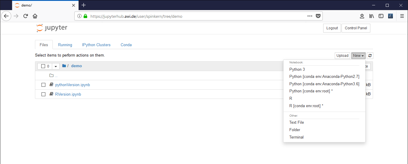
To start a new notebook document click on “New” and select a preinstalled environment.

All input in a notebook document is organized in cells, of which two types exist:

Code cells contain (Python or R) source code and can be executed interactively using the selected kernel. The output is shown below the cell.

Markdown cells contain formatted text. The formatted code replaces the markdown code when the cell is executed.

A cell can be executed by clicking the “Run” button or by the shortcut “CTRL” + “Enter”.

Each code cell gets a sequential number to indicate the order in which the cells have been executed.

The active cell has a colored bar at the left side indicating whether it is in “editing” mode (green) or “command” mode (blue). The modes are switched using the “Esc” and “Enter” key respectively.

Several shortcuts are predefined, e.g. in the command mode:

• Up/down keys: scroll up and down the cells
• A: Create a new cell above the selected one
• B: Create a new cell below the selected one
• M: Treat the active cell as a markdown cell
• R: Raw cell (like a code cell, but won’t be executed)
• Numbers 1-6 Format cell to heading
• Y: Treat the active cell as a code cell
• DD: Delete the active cell
• Z: undo a cell delete
• Shift + M: Merge active and following cell

In edit mode:

• CTRL + Enter: Execute the cell
• CTRL + SHIFT + “-“ (minus): Split the cell at the cursor position

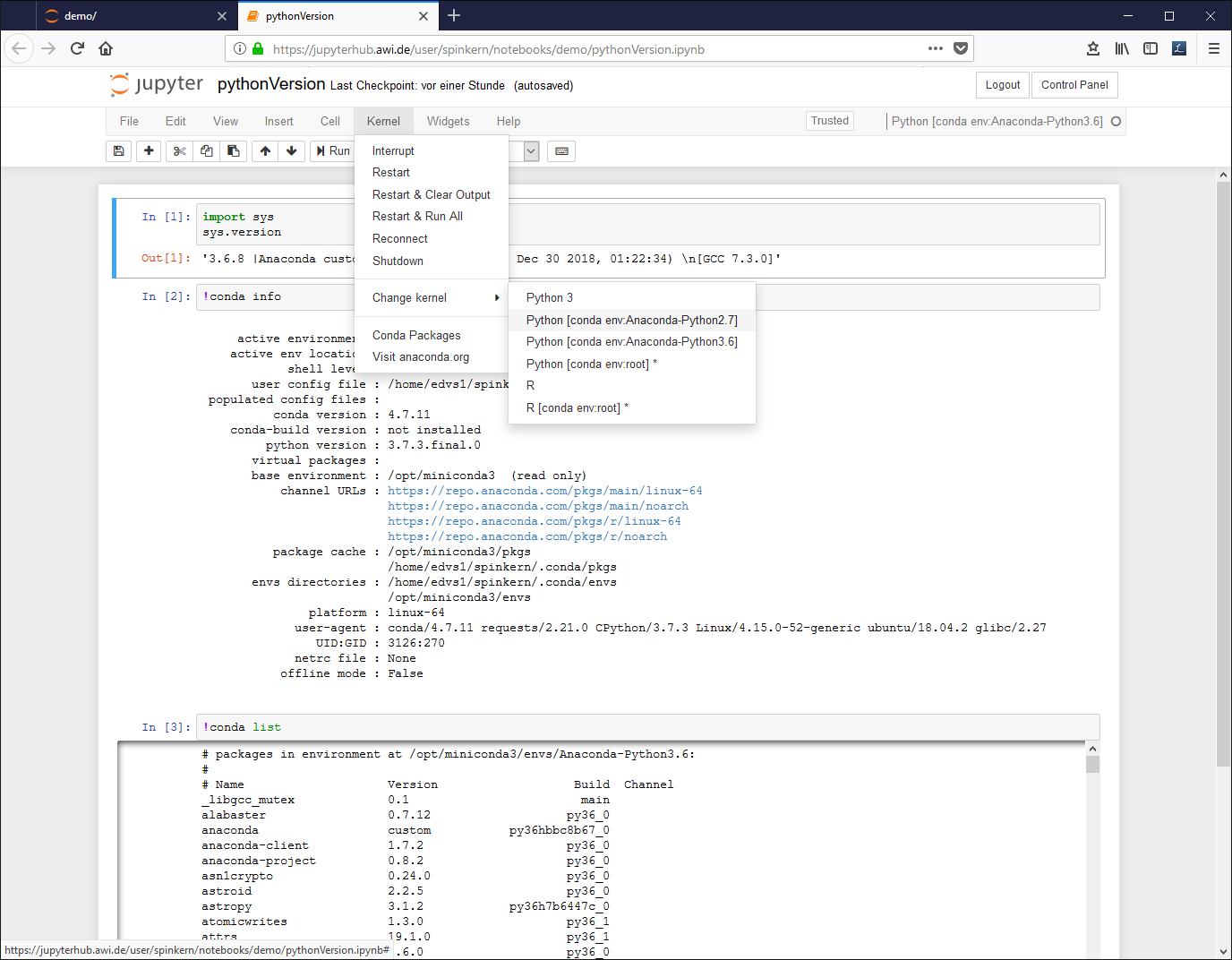
A notebook document needs a connected kernel to be executable. The active kernel is shown in the upper right corner. To change the kernel, click “kernel” à “change kernel” in the menu bar, and select the desired kernel.

Preinstalled kernels are:

• Python [conda env:Anaconda-Python2.7] : Python 2.7 and default libraries (Anaconda)
• Python [conda env:Anaconda-Python3.6] : Python 3.6 and default libraries (Anaconda)
• R : R 3.6 and default libraries

These kernels are read-only! This means users cannot add additional libraries to the kernels. If further libraries are needed, a new environment for own libraries has to be created first.

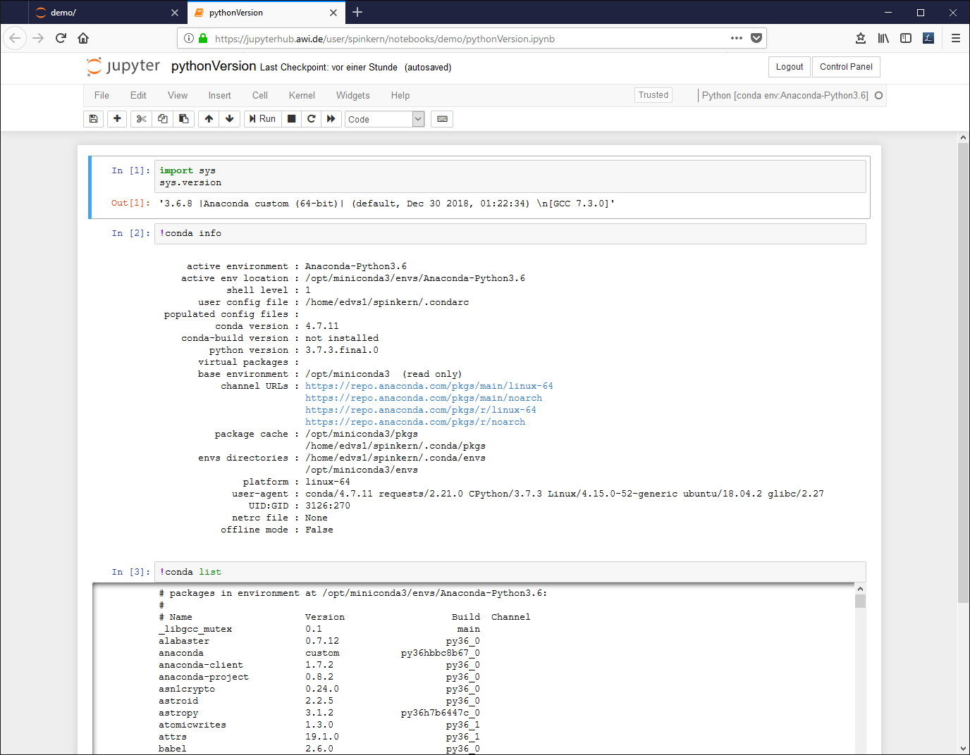
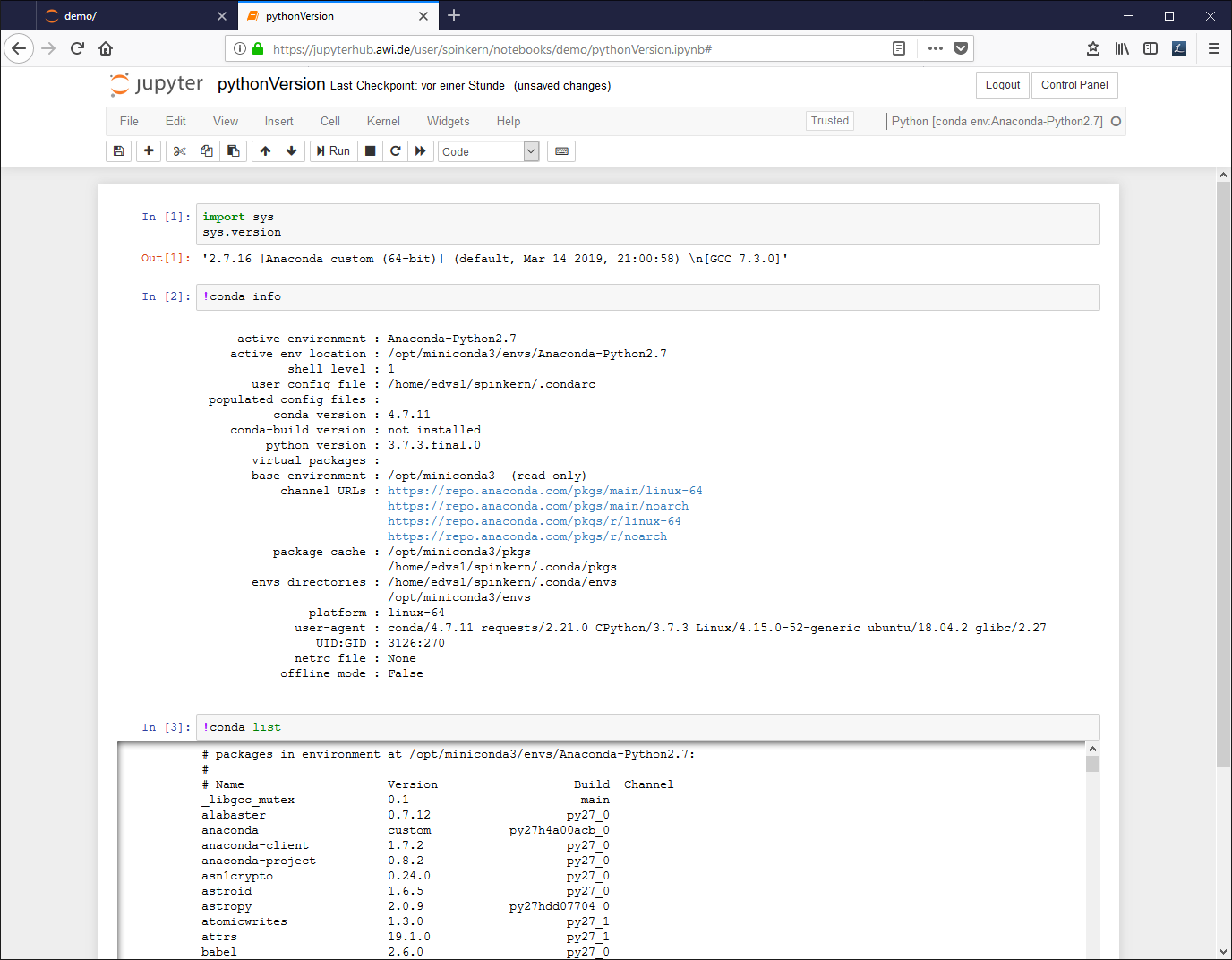
Edit the document. A source code (Python in this case) cell can be executed by pressing CTRL and Enter buttons:

To change the environment, click “Kernel”, “Change kernel”, and select another environment from the list.

Executing the notebook again changes the output:

Terminal

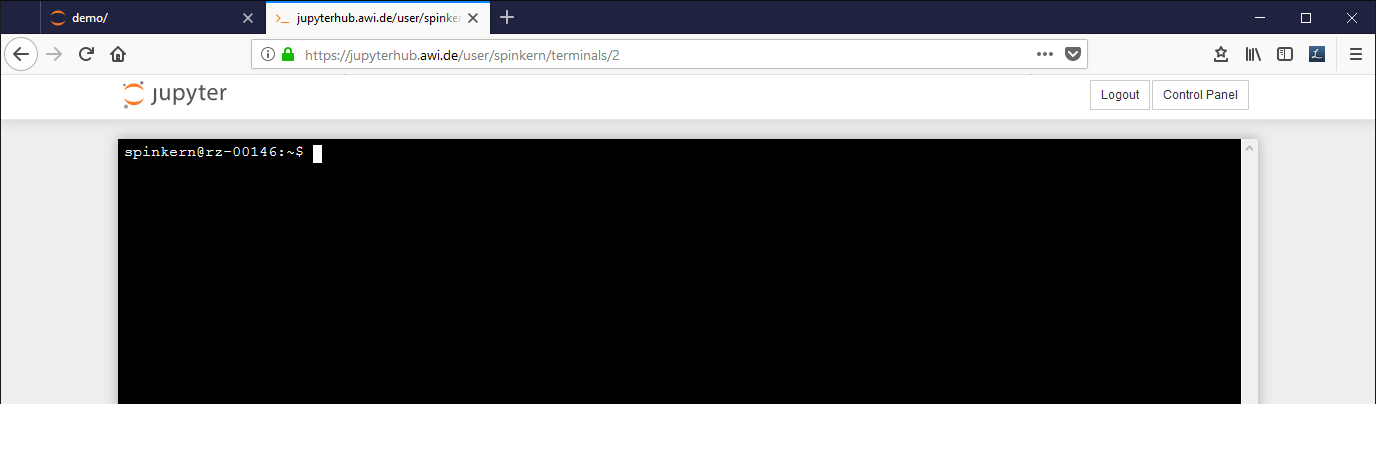
In the “Files” tab, click “New” and “Terminal”.

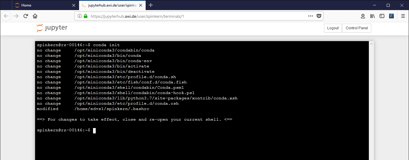
A config tool automatically sets the paths for the conda tools. This has to be activated once by:

            conda init

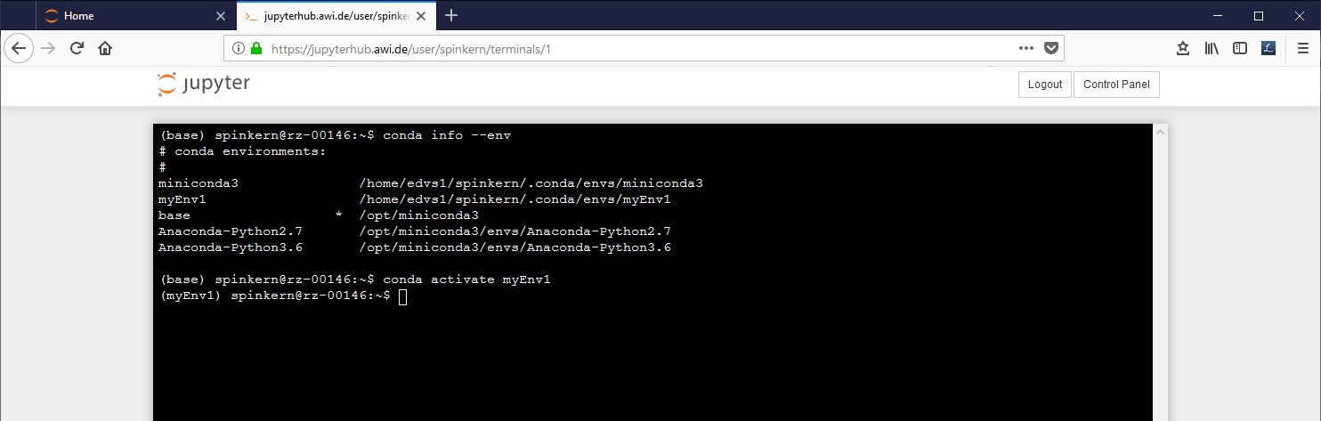
To get a listing of the environments:

            conda info –env

To change the active environment:

            conda activate myEnv1

The active environment is indicated in brackets in the beginning of the line in the terminal.

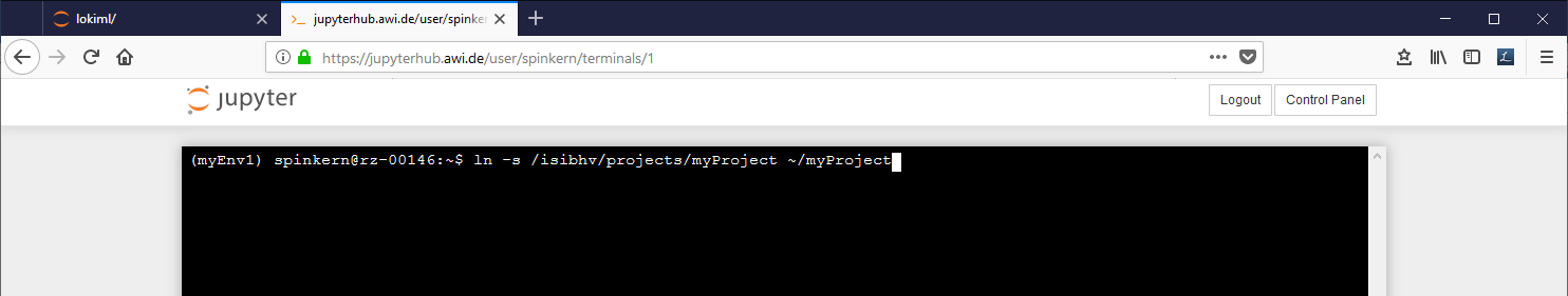
To place a link to the MCS into your home folder type the following commands into the terminal:

cdln -s /isibhv/(…)

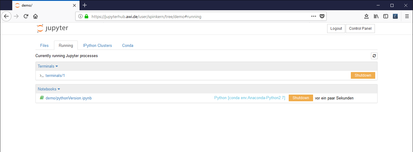
The “Running” tab

This tab gives an overview of running notebook documents, terminals, etc. It is recommended to close all running notebooks, that are not actively used.

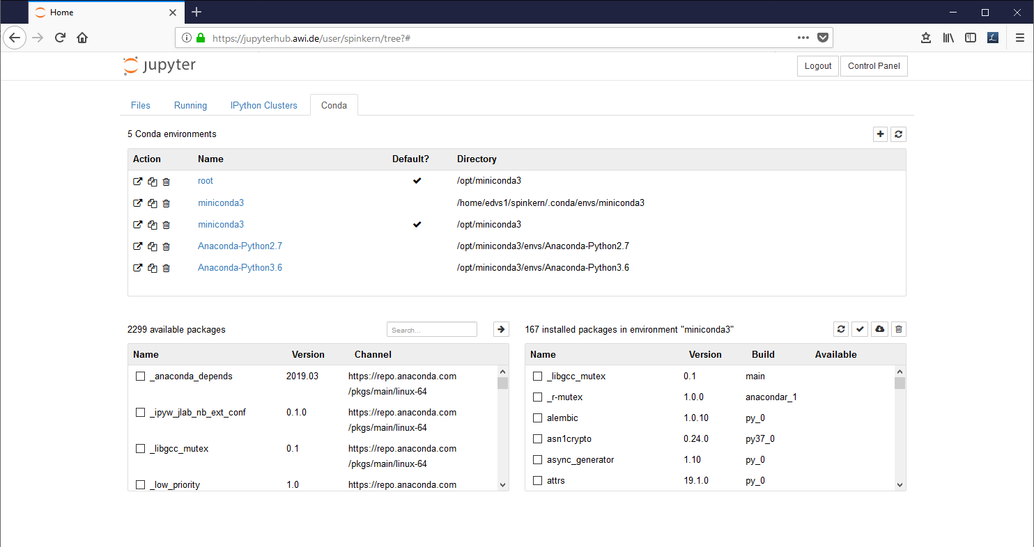
The “Conda” tab

The Conda tab can be used to create new Python 2 and Python 3 environments and to install additional libraries.

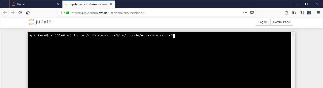
Suppress the error message in the Conda tab

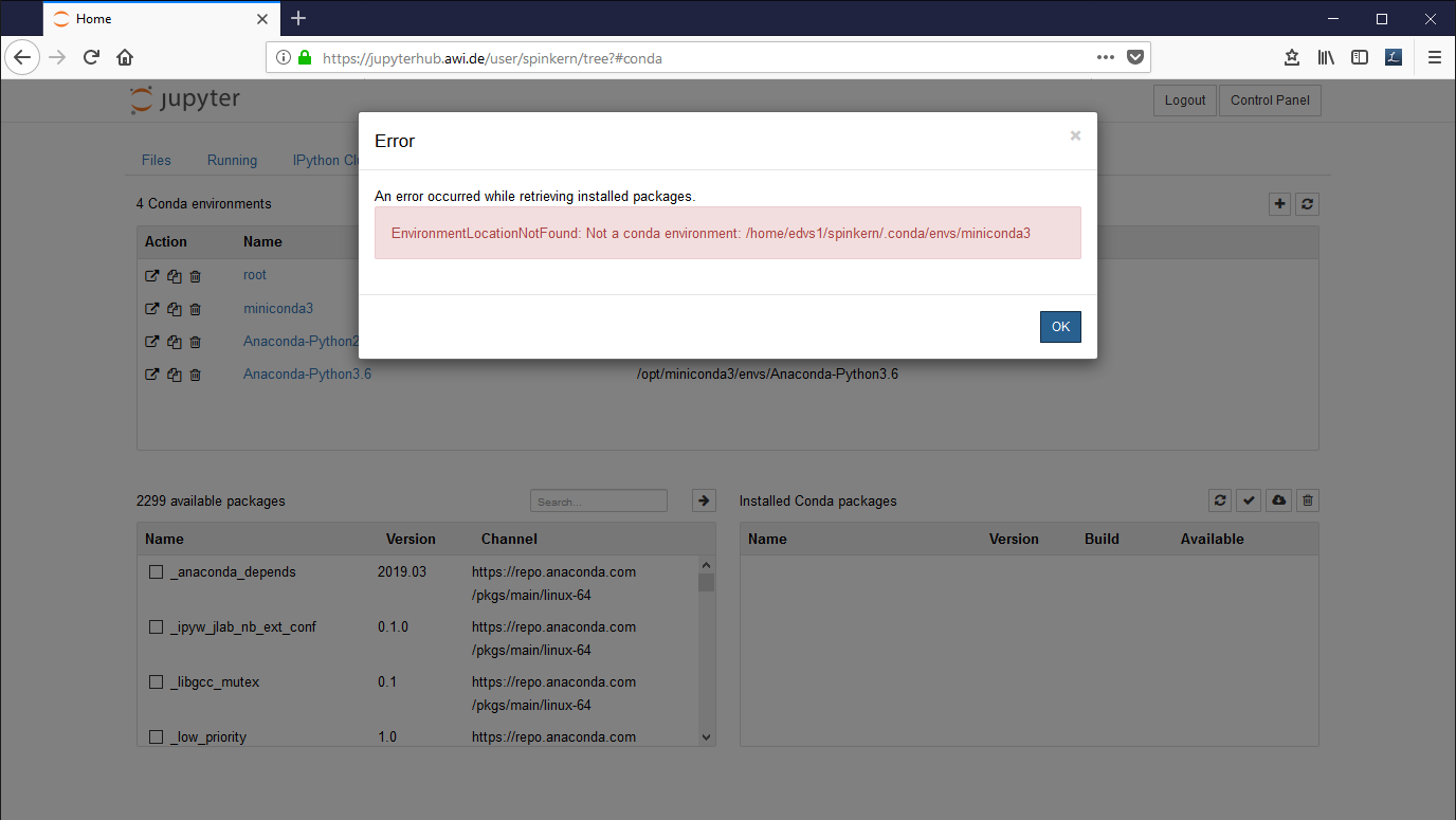
In case you get this error message, execute the following command in the terminal:

ln -s /opt/miniconda3/ ~/.conda/envs/miniconda3

The “Clusters” tab

This option is not supported in this version.

Python

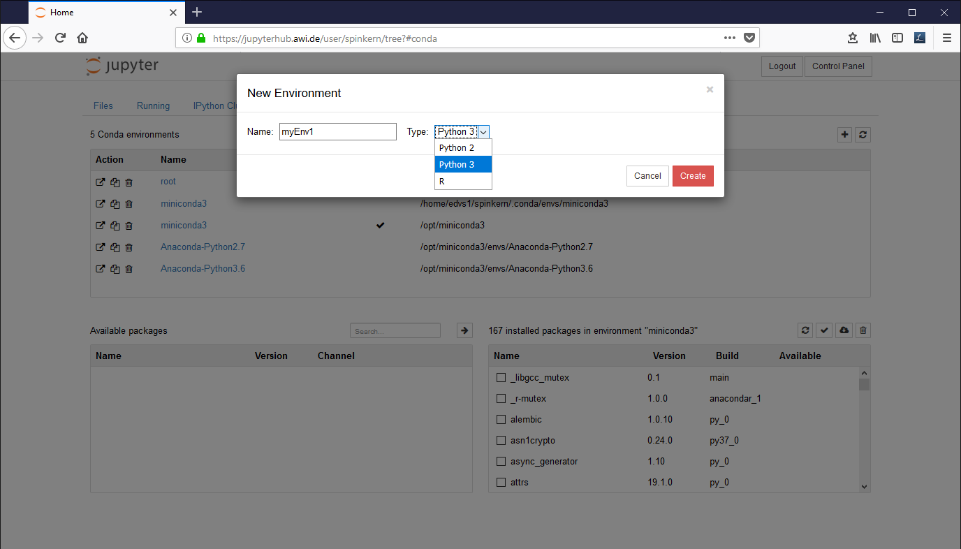
Creating an own Python Environment

In the “conda” tab, click on the plus button in the upper right corner. Set a name for the new environment, select “Python 2” or “Python 3” from the dropdown box, and click “Create”.

Alternatively, a new environment can be created by the conda CLI using the terminal.

Installing Python libraries

The users cannot modify the pre-installed conda environments. So, to install additional libraries, an own environment needs to be created first.

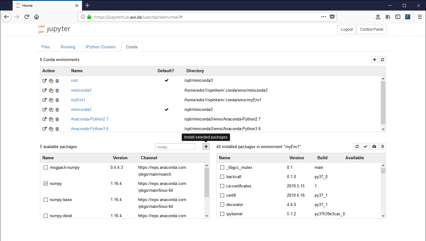
In the "Conda" tab, select the new environment ('myEnv1' in this example).

The installed libraries are listed in the window at the bottom, on the right side. Available packages can be selected in the list at the bottom, left side.

Mark the desired packages and click the Arrow Button to install them. The underlying conda package manager automatically resolves package dependencies.

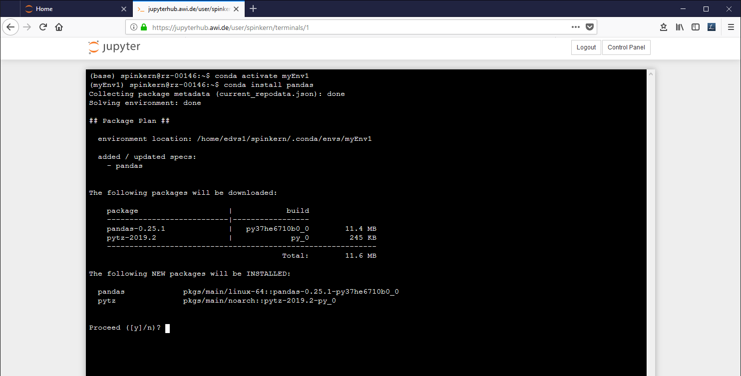
Conda package manager

Instead of using the "Conda" tab mentioned before, you can also use the conda package manager via the terminal. The package manager allows to configure the conda environment, which is the base of the Jupyter Notebook application.

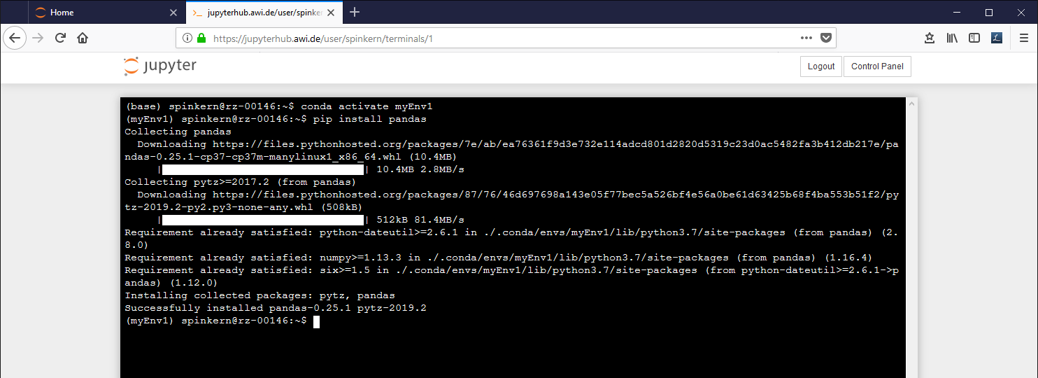
PIP

Most packages are available via the conda package manager, as described below. Alternatively, pip can be used via the terminal.

Please make sure to use the pip version, that belongs to the correct Python environment.

The environments’ version can be found under:  ~/.conda/envs/[envName]/bin/pip

Alternatively, the environment has to be “activated” first, which links the global “pip” command to that of the activated environment.

R

The R environment comes with preinstalled Tidyverse meta-package. Users can add R packages, which will be installed in a personal library in their central home folder. In contrast to the Python environments, no additional environment needs to be created. Additional R libraries can be installed using the install.package() command within R, either using an R notebook or the terminal.

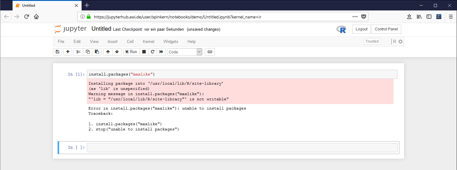
Please note that the install command might fail, if it is submitted from within a notebook document.

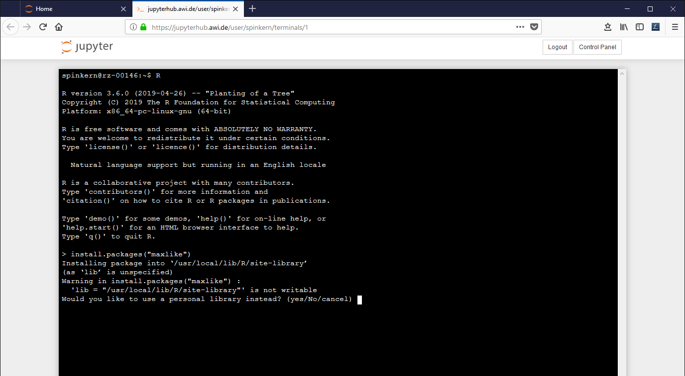
Example: The local library needs to be created before a new package can be installed. Within the notebook, the install command fails, while in the terminal the program asks what to do...

Start the terminal as described above and start the R console by typing "R".

Here, the same install command leads to a dialog, to ask if a personal library shall be used instead.